Continuous Random Variables

Lecture_5 Continuous Random Variables

Contents

Lecture_5

1. PDF & CDF
2. Uniform Distribution
3. Basic Monte Carlo Simulation
4. Exponential Distribution
5. Normal Distribution
6. Central Limit Theorem
7. Moment Generating Functions

PDF&CDF

• Definition

For a continuous r.v. $X$ with CDF $F$ , the probability density function(PDF) of $X$ is the derivative f of the CDF, given by $f (x) = F’(x)$.The support of $X$, and of its distribution, is the set of all $x$ where $f (x) > 0$.

\begin{cases}
PMF: & P(X=x),prob \in [0,1]\\
PDF: & f(x) \neq prob = \int_A f(x)dx\\
\end{cases}
So, $f(x) > 1$ Could be!!
if $X$ is a continuous $r.v.$ $P(X=a) = 0, \forall a\in R$

• PDF to CDF

Let $X$ be a continuous $r.v.$ with PDF $f$ . Then the CDF of $X$ is given
by
$$
F(X) = \int_{-\infty}^\infty f(t)dt
$$

• Valid PDF

1. Nonnegative: $f(x) \geq 0$
2. Intergrates to 1: $\int_{-\infty}^\infty f(x)dx = 1$

Expectation of A continuous R.v

• Definition
  $$
  E(x) = \int_{-\infty}^\infty xf(x)dx
  $$

$$
\begin{equation}
\begin{gathered}
\text{LOTUS: }
E(g(x)) = \int_{-\infty}^\infty g(x)f(x)dx\\
\text{For Survival Function: } G(x) = 1-F(X) = P(X>x)\\
E(x) = \int_{0}^\infty G(x)dx
\end{gathered}
\end{equation}
$$

Uniform Distribution

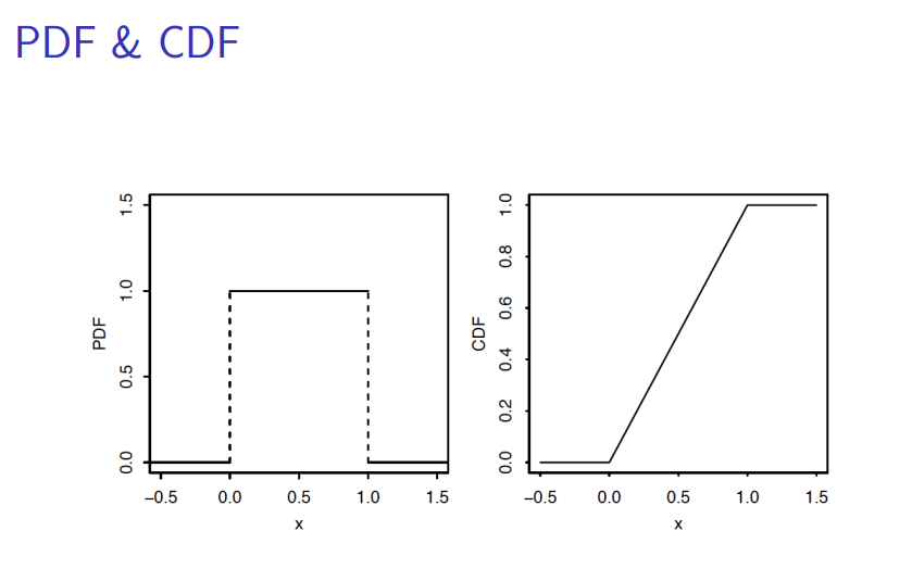
E.G
Suppose $X_1, X_2,\cdots, X_n$ are i.i.d Unif(0, 1) random variables and let
$Y = min(X_1, X_2,\cdots, X_n)$ be their minimum. Find $E(Y)$.

▶

Solution

Basic Monte Carlo Simulation

• Theorem
  1. Let $U \sim Unif (0, 1)$ and $X = F^{-1}(U)$. Then $X$ is an $r.v.$ with CDF $F$.
  2. Let $X$ be an $r.v.$ with CDF $F$. Then $F(X) \sim Unif (0, 1)$.

More proof for Universality around $P.30$.

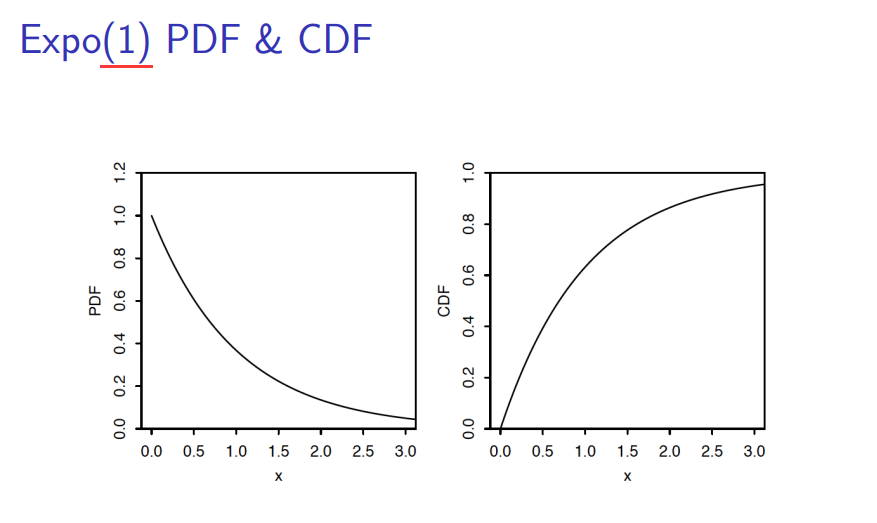
⭐Exponential Distribution

A continuous $r.v. X$ is said to have the Exponential distribution with
parameter $\lambda$ if its PDF is
$$
f(x) = \lambda e^{-\lambda x},x>0
$$
And
$$
\begin{align}
\text{CDF: }F(x) &= 1-e^{-\lambda x},x>0\\
\text{Survival Function: } G(x) &= 1-F(x) = e^{-\lambda x},x>0
\end{align}
$$

Memoryless Property

A distribution is said to have the memoryless property if a random
variable X from that distribution satisfies
$$
P (X ≥ s + t|X ≥ s) = P (X ≥ t)
$$

If $X$ is a positive continuous random variable with the memoryless
property, then $X$ has an Exponential distribution.

Proof around $P.44$

E.G
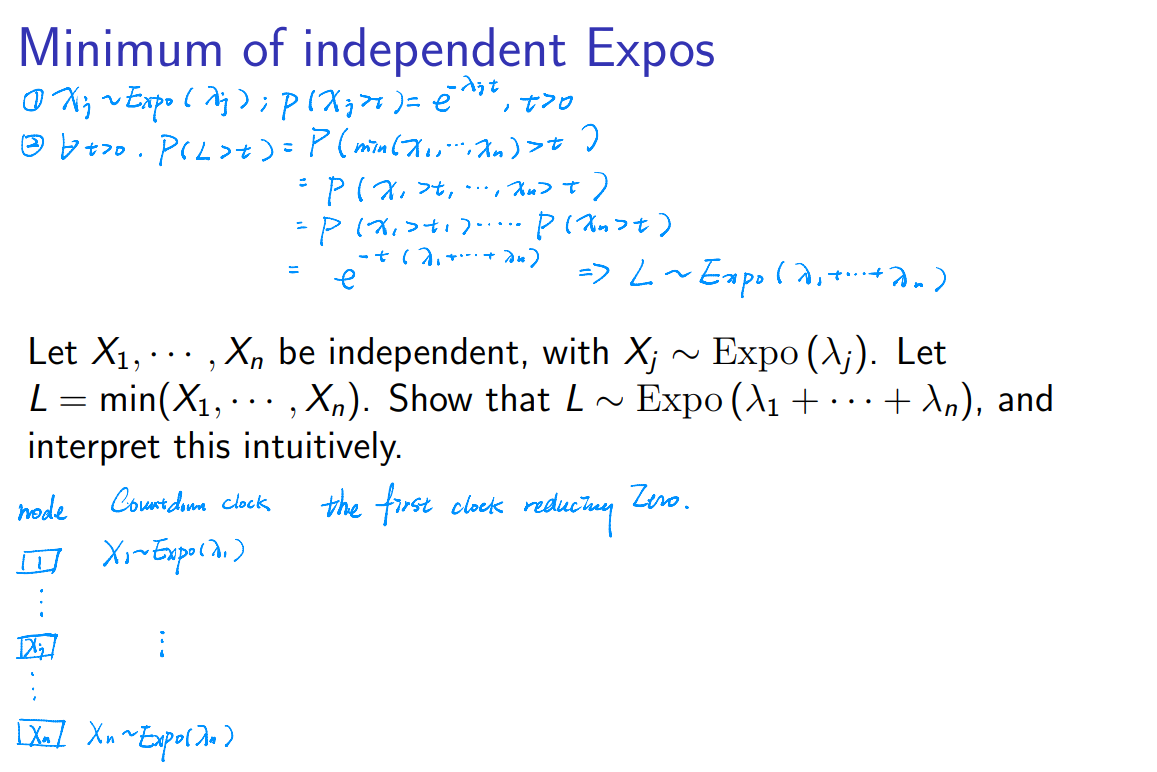
Minimum of independent Expos
Let $X_1,\cdots, X_n$ be independent, with $X_j ∼ Expo(λ_j)$. Let
$L = min(X_1,\cdots, X_n).$ Show that $L ∼ Expo (λ_1 +\cdots+ λ_n)$, and
interpret this intuitively.

▶

Solution

Failure (Hazard) Rate Function

Let $X$ be a continuous random variable with pdf $f(t)$ and CDF
$F(t) = P(X ≤ t)$. Then the failure (hazard) rate function $r(t)$ is
$$
r(t) = \frac{f(t)}{1-F(t)}
$$

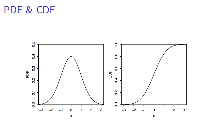
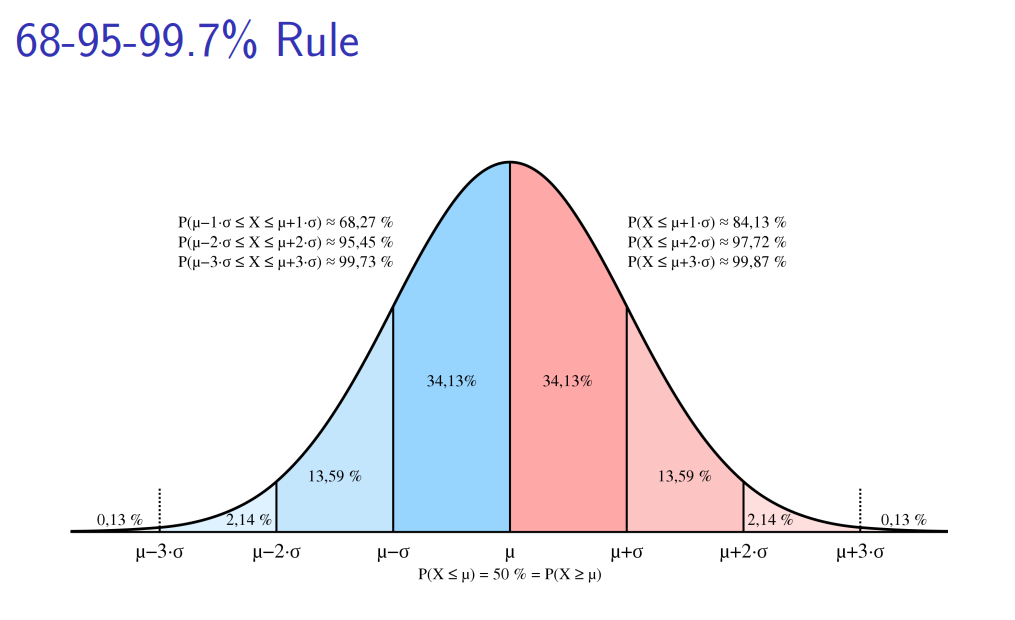
⭐⭐Normal Distribution

standard Normal distribution

For standard Normal distribution $Z\sim N(0,1)$ , whose mean is 0 and variance is 1:
$$
\begin{align}
PDF: \varphi(z) &= \frac{1}{\sqrt{2\pi}}e^{-z^2/2}\\
CDF: \Phi(z) &= \int_{-\infty}^z\varphi(t)dt=\int_{-\infty}^z\frac1{\sqrt{2\pi}}e^{-t^2/2}dt
\end{align}
$$

• $\varphi$ for the standard Normal PDF, $\Phi$ for the CDF and Z for the
  $r.v.$
• Symmetry of tail areas: $\Phi(z)=1-\Phi(-z).$
• Symmetry of $Z$ and $-Z$: If $Z\sim\mathcal{N}(0,1)$, then $-Z\sim\mathcal{N}(0,1)$.
• Mean is 0 and variance is 1.

Normal distribution

• definition
  If $Z\sim\mathcal{N}(0,1)$, then
  $$
  X=\mu+\sigma Z
  $$
  is said to have the Normal distribution with mean $\mu$ and variance $\sigma^{2}$. We denote this by $X\sim\mathcal{N}(\mu,\sigma^2).$

• Theorem
  Let $X\sim \mathcal{N}(\mu,\sigma^2)$. Then the CDF of $X$ is
  $$
  F\left(x\right)=\Phi\left(\frac{x-\mu}\sigma\right)
  $$
  and the PDF of $X$ is
  $$
  f\left(x\right)=\varphi\left(\frac{x-\mu}\sigma\right)\frac1\sigma
  $$

Central Limit Theorem

• Definition of Sample Mean
  Let $X_1,…,X_n$ be i.i.d. random variables with finite mean $\mu$ and finite variance $\sigma^2$. The sample mean $\bar{X}_n$ is defined as follows:
  $$
  \bar{X}_n=\frac{1}{n}\sum_{j=1}^nX_j
  $$
  The sample mean $\bar{X}_n$ is itself an r.v. with mean $\mu$ and variance $\sigma^2/n.i.e.,\bar{X}_n\sim \mathcal{N}(\mu,\sigma^2/n)$

• Central Limit Theorem
  As $n\to\infty$,
  $$
  \sqrt{n}\left(\frac{\bar{X}_n-\mu}\sigma\right)\to\mathcal{N}\left(0,1\right) \text{ in distribution}.$$
  In words, the CDF of the left-hand side approaches the CDF of the standard Normal distribution.

• CLT Approximation

  • For large $n$, the distribution of $\bar{X}_n$ is approximately $N(\mu,\sigma^2/n).$
  • For large $n$, the distribution of $n\bar{X}_n=X_1+\ldots+X_n$ is approximately $\mathcal{N}(n\mu,n\sigma^2).$

Poisson Convergence to Normal

Let $Y\sim Pois(n)$. We can consider Y to be a sum of $n$ i.i.d. Pois(1) r.v.s. Therefore, for large $n$,

$$
Y\sim\mathcal{N}(n,n)
$$

Binomial Convergence to Normal

Let $Y\sim Bin(n,p)$. We can consider $Y$ to be a sum of $n$ i.i.d. Bern(p) r.v.s. Therefore, for large $n$,

$$
Y\sim\mathcal{N}(np,np(1-p)).
$$

Continuity Correction: De Moivre-Laplace Approximation

\begin{aligned}
P(Y=k)& =P(k-\frac12<Y<k+\frac12) \\
&\approx\Phi(\frac{k+\frac12-np}{\sqrt{np(1-p)}})-\Phi(\frac{k-\frac12-np}{\sqrt{np(1-p)}}).
\end{aligned}

• Poisson approximation: when $n$ is large and $p$ is small.
• Normal approximation: when $n$ is large and $p$ is around 1/2.

De Moivre-Laplace Approximation

\begin{aligned}
\mathbb{P}(k\leq Y\leq1)& =P(k-\frac12<Y<I+\frac12) \\
&\approx\Phi(\frac{l+\frac{1}{2}-np}{\sqrt{np(1-p)}})-\Phi(\frac{k-\frac{1}{2}-np}{\sqrt{np(1-p)}})
\end{aligned}

• Very good approximation when $n ≤ 50$ and p is around 1/2.

Family of Normal Distribution

Given ii.d. r.v.s $X_i\sim\mathcal{N}(0,1),Y_j\sim\mathcal{N}(0,1),i=1,\ldots,n$, $j=1,\ldots,m$. Then we have

• Chi-Square Distribution
  $$
  \chi_n^2=X_1^2+\ldots+X_n^2$$
• Student-t Distribution
  $$
  t=\frac{Y_1}{\sqrt{\frac{X_1^2+…+X_n^2}n}}$$
• F-distribution:
  $$
  F=\frac{\frac{X_1^2+…+X_n^2}n}{\frac{Y_1^2+…+Y_m^2}m}
  $$

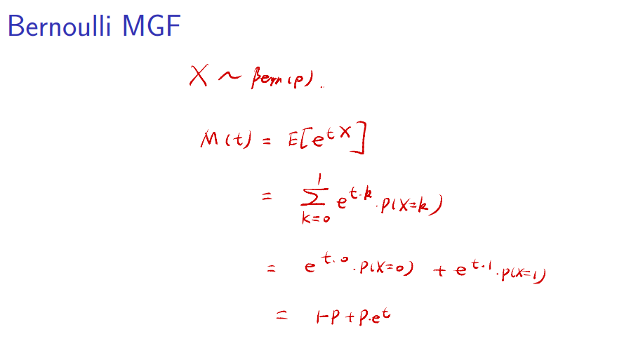
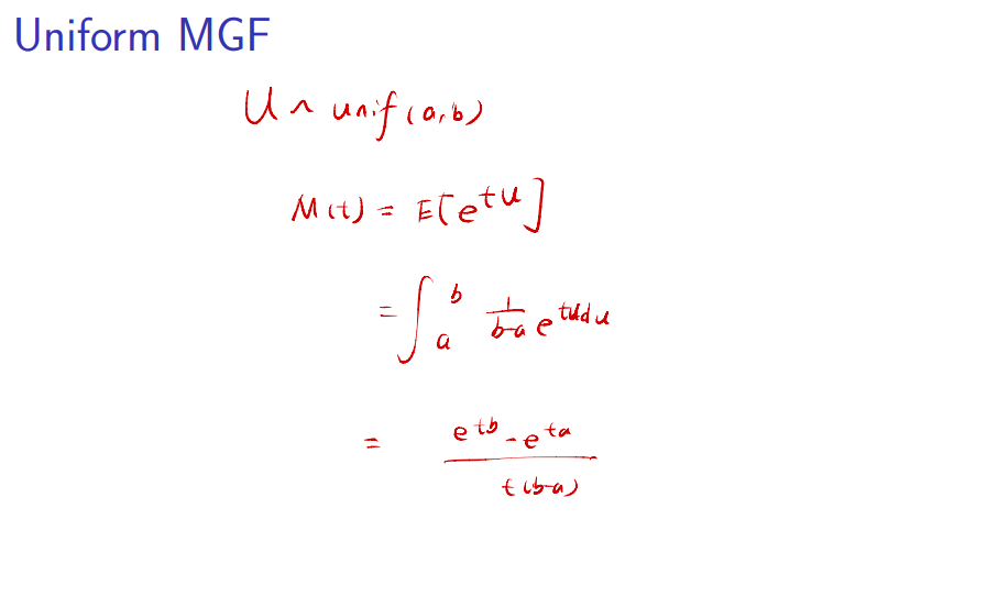
Moment Generating Function

• Definition
  The moment generating function (MGF) of an r.v. $X$ is $M(t)=E(e^{tX})$, as a function of $t$, if this is finite on some open interval $(-a,a)$ containing 0. Otherwise we say the MGF of $X$ does not exist.

E.G

Moments via Derivatives of the MGF

• Theorem
  Given the MGF of X, we can get the n$^{th}$ moment of X by evaluating the n$^{th}$ derivative of the MGF at 0: $E(X^n)=M^{(n)}(0).$

MGF of A Sum of Independent R.V.s

• Theorem
  If X and Y are independent, then the MGF of $X+Y$ is the product of the individual MGFs:
  $$
  M_{X+Y}\left(t\right)=M_X\left(t\right)M_Y\left(t\right).
  $$

E.G

MGF of Location-scale Transformation

• Theorem
  If $X$ has MGF $M(t)$, then the MGF of $a+bX$ is
  $$
  E\left(e^{t(a+bX)}\right)=e^{at}E\left(e^{btX}\right)=e^{at}M\left(bt\right).
  $$

See more examples in Lecture_5